The best way to read the textbook is to do some of the exercises. I expect you to spend 6 to 9 hours doing so outside of class each week. This is based on the popular rule of thumb that three class hours implies six to nine study hours.
Let’s look at some of the Chapter 1 exercises briefly.
2.2 Textbook Section 1.1, An Example Experiment (stents)
Here we looked at treatment groups and control groups.
2.2.1 Textbook Exercise 1.1, the migraine data set
In class we loaded the data set and made a contingency table, with which we can answer the four questions in Exercise 1.1.
         group
pain_free control treatment
      no       44        33
      yes       2        10
The four questions are:
What percent of patients in the treatment group were pain free 24 hours after receiving acupuncture?
What percent were pain free in the control group?
In which group did a higher percent of patients become pain free 24 hours after receiving acupuncture?
Your findings so far might suggest that acupuncture is an effective treatment for migraines for all people who suffer from migraines. However, this is not the only possible conclusion that can be drawn based on your findings so far. What is one other possible explanation for the observed difference between the percentages of patients that are pain free 24 hours after receiving acupuncture in the two groups?
We can use the tbl object we created to answer these questions.
The percentage of patients in the treatment group who were pain free was 23.3%.
The percentage of patients in the control group who were pain free was 4.3%.
A higher percent of the treatment group became pain free.
Not all migraine headaches are alike. It is possible that, due to chance, the patients in the treatment group had less severe migraine headaches that were easier to cure.
Examine the .qmd file that renders into this .html file. You’ll see that, rather than specify the numbers in the answers above, we actually did the calculations inline. What is good about doing this? (Hint: what happens if you add patients to the data set and rerender the document?) What is bad about doing this? (Hint: it looks clumsy and we could just as easily run the calculations in an r chunk, assign the results to object, and name the objects inline.)
Another issue is the code for part c. I only accounted for the case where the treatment group has the greater percent. It would be much better to add an else clause to account for the possibility that the answer should be control and an else to account for the two to be equal. The best way to do that is to create a non-echoing chunk and use the results inline. For example, the following chunk only appears in the .qmd file, not the .html file, but its results can be used inline.
Now we can say that the treatment group had the higher percentage. Only one problem remains and it is a software engineering problem. We haven’t tested the above code on a case where the control group or neither group had the higher percentages. We’ll leave that for now as a more advanced topic.
2.3 Textbook Section 1.2, Data Basics
Here we looked at
observations (rows), variables (columns), and data matrices (data frames)
types of variables (dbl or continuous, int or discrete, fctr or nominal, and ordered fctr or ordinal)
relationships between variables
explanatory (x or features or input) and response (y or targets or output) variables
observational studies and experiments (and we mentioned an in-between activity called quasi-experiments)
Data Type terminology: R vs the Textbook
R
Openintro Stats textbook
dbl, as.numeric()
numerical, continuous
int, as.integer()
numerical, discrete
fctr, factor()
categorical, nominal
ord, ordered()
categorical, ordinal
On the left of the above table, you see how R refers to data types. On the right is how the OpenIntro Stats textbook refers to data types. When you display a tibble (a tibble is a data frame with some extra information) using R, each variable column will be headed with dbl, int, fctr, or ord to indicate the four kinds of numbers. If a variable is not interpreted as a number, R will display chr as an abbreviation of character.
2.3.1 Textbook Exercise 1.7
What were the explanatory and response variables in the migraine study? The group was explanatory and pain_free was the response variable.
2.3.2 Textbook Exercise 1.12
This is a hard question in two parts.
List the variables used in creating this visualization.
Indicate whether each variable in the study is numerical or categorical. If numerical, identify as contin- uous or discrete. If categorical, indicate if the variable is ordinal.
There is actually an r package underlying this question. If you visit https://github.com/dgrtwo/unvotes you will see the data represented as a tibble. If you recall, during week one we said that a tibble is a data frame that behaves well. Among its features is a list of the data types, so you can answer parts a and b by looking at a tibble of the data, where you’ll see that
year is stored as dbl although it is really discrete and could be stored as int
country is stored as chr which means characters although it is really a nominal factor
percent_yes is stored as a dbl which is appropriate
issue is stored as chr although it is really a nominal factor
Later we’ll learn how to produce a visualization like this, although you are welcome to try based on the code at the unvotes website mentioned above. If you want the actual code itself, you can slightly modify the code at https://rpubs.com/minebocek/unvotes to include Mexico.
2.4 Textbook Section 1.3, Sampling
Here we talked about random sampling, stratified sampling, cluster sampling, and observational studies.
2.4.1 Textbook Exercise 1.15, Asthma
What is the population of interest and the sample? Note that the population is NOT all asthma sufferers. The population of interest is all asthma patients aged 18-69 who rely on medication for asthma treatment. The sample consists of 600 such patients.
Is the study generalizable? Can we establish cause and effect? The patients are probably not randomly sampled, so we need to know more to say whether they represent all asthma patients 18–69 who rely on medication. For example, they could all be from a high-pollution city. We would need to know that. The cause and effect determination is easier. An experiment can determine cause and effect, while an observational study only determines association.
2.5 Textbook Section 1.4, Experiments
Here we discussed four issues:
control
randomization
replication
blocking
2.5.1 Textbook Exercise 1.34, Exercise and mental health
A researcher is interested in the effects of exercise on mental health and he proposes the following study: Use stratified random sampling to ensure representative proportions of 18-30, 31-40 and 41-55 year olds from the population. Next, randomly assign half the subjects from each age group to exercise twice a week, and instruct the rest not to exercise. Conduct a mental health exam at the beginning and at the end of the study, and compare the results.
What type of study is this?
What are the treatment and control groups in this study?
Does this study make use of blocking? If so, what is the blocking variable?
Does this study make use of blinding?
Comment on whether or not the results of the study can be used to establish a causal relationship between exercise and mental health, and indicate whether or not the conclusions can be generalized to the population at large.
Suppose you are given the task of determining if this proposed study should get funding. Would you have any reservations about the study proposal?
2.5.2 Answers
This is an experiment.
The treatment is exercise twice a week and control is no exercise.
Yes, the blocking variable is age.
No, the study is not blinded since the patients will know whether or not they are exercising.
Since this is an experiment, we can make a causal statement. Since the sample is random, the causal statement can be generalized to the population at large. However, we should be cautious about making a causal statement because of a possible placebo effect.
It would be very difficult, if not impossible, to successfully conduct this study since randomly sampled people cannot be required to participate in a clinical trial
2.6 Textbook Chapter 2: Summarizing data
This week, we’ll look at numerical data, categorical data, and a case study.
2.6.1 Numerical data
There are graphical and numerical methods for summarizing numerical data, including
scatterplots
dot plots
mean
histograms
variance and standard deviation
box plots, quartiles, and the median
robust statistics
cartographic maps and cartograms
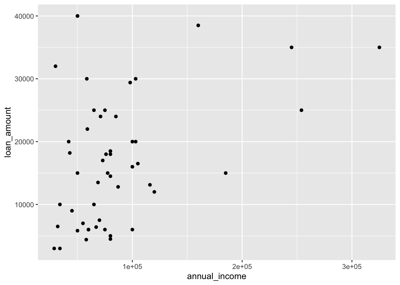
We can draw a scatterplot of two variables of the loan50 data as follows.
The above is a very basic scatterplot. Later, we’ll learn to change colors, background, labels, legends, and more. Bear in mind that the scatterplot is meant to compare two numeric variables. You can’t use it for a numeric variable and a categorical variable.
A dotplot may be helpful to illustrate a categorical variable, but I seldom use them. Using them in concert with a boxplot may make more sense. We’ll look at boxplots later.
The mean is part of a good summary of data. We can find the mean of a variable by saying mean(variable_name) or as part of a summary. For instance
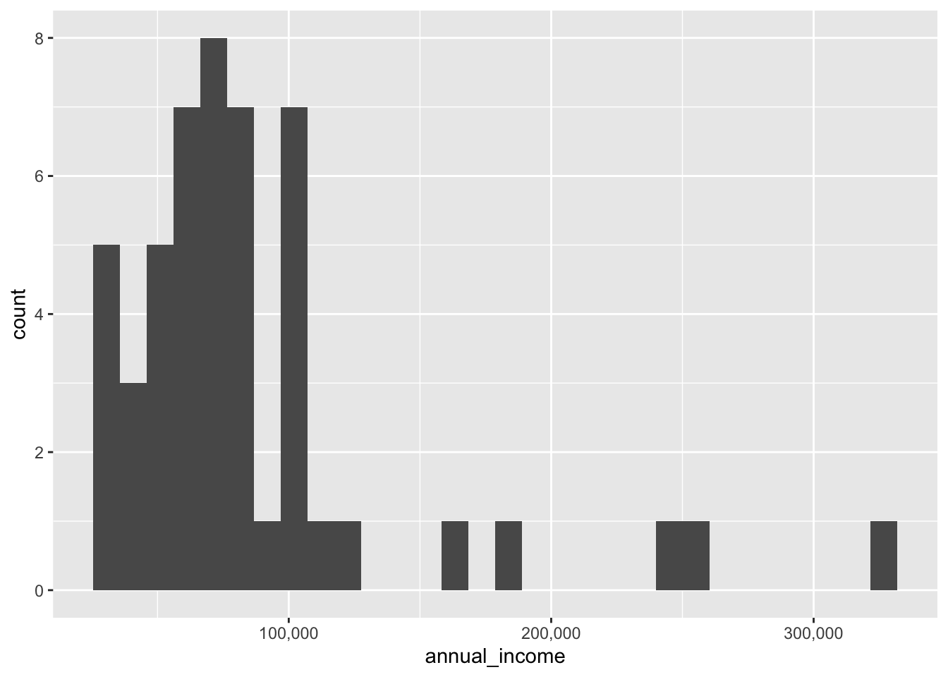
with(loan50,mean(annual_income))
[1] 86170
with(loan50,summary(annual_income))
   Min. 1st Qu.  Median    Mean 3rd Qu.    Max.
  28800   55750   74000   86170   99500  325000
Notice that the summary() function also gives us the minimum, the first quartile, the median, the 3rd quartile, and the maximum value of the variable, in addition to the mean. We’ll discuss all these statistics in the context of other ways to extract them. The problem with the mean that is demonstrated in the textbook is that two variables may have very different shapes but the same mean. So the textbook then describes histograms, which are a good way to identify the shape of a variable.
Notice that the x-axis labels are shown in scientific notation. We can fix this using the scales package. By the way, in case I haven’t mentioned it before, we always refer to the horizontal axis as the x-axis and the vertical axis as the y-axis. This is the default for r and many other languages that create graphical displays.
You may have noticed that Hadley Wickham, the inventor of the Tidyverse, dislikes the default number of bins in a histogram. So he programmed ggplot() to always show a warning message saying to pick a better number, depending on your data. We can fix that easily with a parameter to geom_histogram(). Then each bin (vertical stripe) will represent a thousand dollars.
You may notice that warning messages aren’t dealbreakers. An error message on the other hand, will often stop output dead in its tracks.
The next concepts covered in the textbook are variance and standard deviation. We can calculate them as follows. When you do this, you may notice that sd() is the square root of var(). Why would you prefer one over the other? Usually you use sd() because it’s in the same units as the data, dollars in the following case, unlike var(), which is in squared units, squared dollars in the following case.
with(loan50,var(annual_income))
[1] 3e+09
with(loan50,sd(annual_income))
[1] 57566
Together, the mean and standard deviation are often a good, yet compact, description of a data set.
You may want to find the means of all the columns in a data set. If you try to do that with the colMeans() function, you’ll get an error message as follows. (Actually, I’ve disabled the following code chunk by saying #| eval: false in the .qmd file because otherwise the rendering would halt.)
colMeans(loan50)
The remedy is to use a logical function to identify only the numeric columns.
Notice that you often wrap a function inside another function. The only problem is that it’s easy to lose track of all the parentheses.
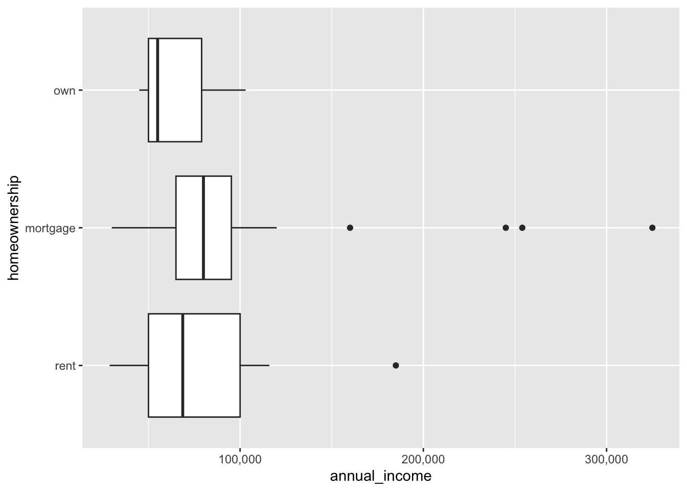
The next topic in the textbook is the box plot. This also gives an opportunity to talk about the quartiles and the median. We can display a box plot as follows.
The thick line in the middle of the box is the median, the middle value of the data set. The box itself is bound by the first and third quartiles, known as hinges. The full name of this construct is actually a box and whiskers plot and the lines extending horizontally from the box are called whiskers. The upper whisker extends from the hinge to the largest value no further than 1.5 * IQR from the hinge (where IQR is the inter-quartile range, or distance between the first and third quartiles). The lower whisker extends from the hinge to the smallest value at most 1.5 * IQR of the hinge. Data beyond the end of the whiskers are called “outlying” points and are plotted individually.
We often want to create several box plots and compare them. This is easy to do as follows.
The textbook’s next topic is Robust Statistics and we’re going to pretty much skip that for now, except to say that outliers, as shown in the textbook, can affect the value of some statistics more than others. The mean and median are a good example. The median is much more robust to outliers than is the mean, which can be dragged way up or down by the presence of just one or a few outliers, whereas the median can not. As a kind of thought experiment, consider the following data set and the addition of an outlier and the effect of the outlier on the mean and median.
x<-c(2,3,3,3,4,4,4,5,5,6,6)mean(x)
[1] 4
median(x)
[1] 4
y<-c(2,3,3,3,4,4,4,5,5,6,6,800)mean(y)
[1] 70
median(y)
[1] 4
2.7 Uncertainty in summaries
How can we portray our uncertainty about estimates of parameters? Consider two different vectors:
u <-c(1,2,3,4,5,6,7,8,9)v <-c(3,4,5,5,5,5,5,6,7)
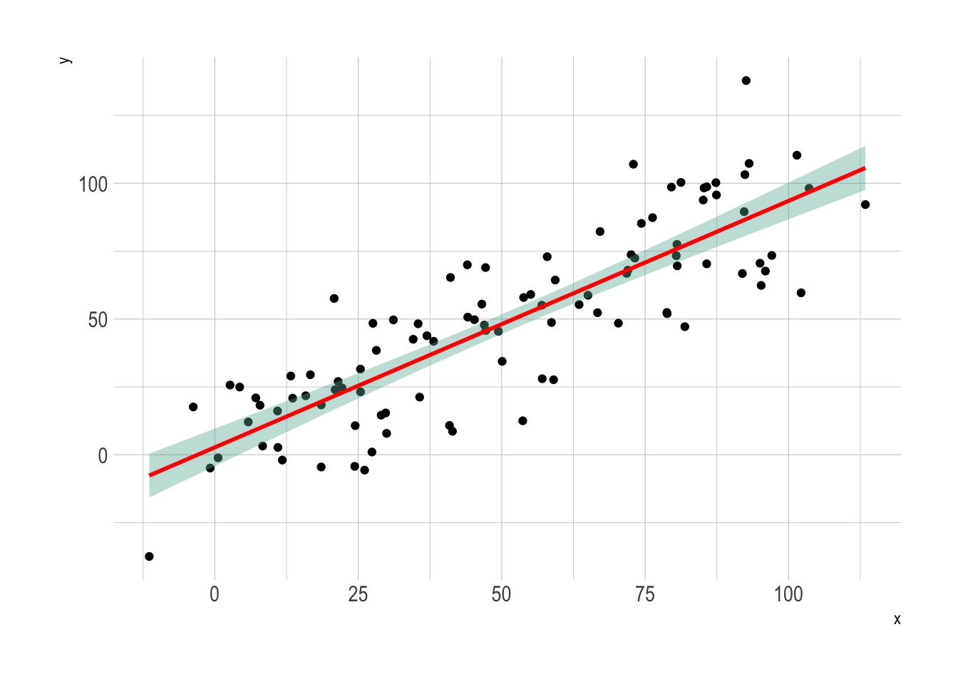
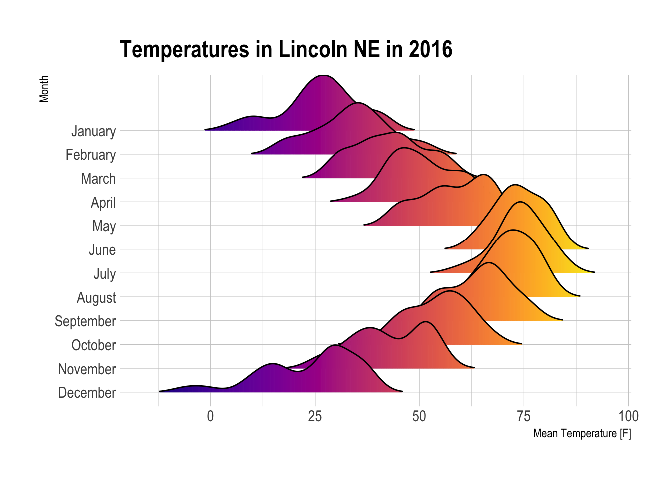
Suppose that these are samples from two different populations. For both of these vectors, the best estimate is 5. Both the mean and median are 5 in both cases. But when estimating, we’re much more sure of our estimate in the case of v than u. We quantify that with variance or its square root, standard deviation. But those numbers don’t mean much to most people. It’s easier to portray uncertainty graphically than numerically. The typical ways to do so are to make boxplots, violin plots, or barcharts with error bars if we’re comparing two or more groups. If we are estimating a continuous variable, say \(y\), at many different values of \(x\), we can show our uncertainty by estimating standard deviation for portions of the data and putting them together as follows in an example from the R Graph Gallery.
Notice that the confidence interval is narrower at the center than at the extremes. Why? It’s because we’re using more data to estimate at the center and have less uncertainty at the center than at the ends, where the data is truncated.
Suppose we’re doing something even more sophisticated, such as comparing groups of continuous \(y\) variables. A ridgeline plot is a popular solution to show variability, which is often similar to uncertainty, as shown in this example from the R Graph Gallery.
#. packagespacman::p_load(ggridges)pacman::p_load(viridis)#. Plotggplot(lincoln_weather, aes(x =`Mean Temperature [F]`, y =`Month`, fill = ..x..)) +geom_density_ridges_gradient(scale =3, rel_min_height =0.01) +scale_fill_viridis(name ="Temp. [F]", option ="C") +labs(title ='Temperatures in Lincoln NE in 2016') +theme_ipsum() +theme(legend.position="none",panel.spacing =unit(0.1, "lines"),strip.text.x =element_text(size =8) )
Warning: The dot-dot notation (`..x..`) was deprecated in ggplot2 3.4.0.
ℹ Please use `after_stat(x)` instead.
Not only are the temperatures higher in the summer than in the winter, they are less variable, so we’re more certain of what the temperature might be on any given day in summer.
2.8 Categorical Data
We’ve already seen contingency tables and how to manipulate them, which are introduced in more detail in this section. We’ve also seen a mosaic plot. Another kind of plot introduced in this section is the bar plot. We’ll examine each of these.
load(paste0(Sys.getenv("STATS_DATA_DIR"),"/migraine.rda"))tbl <-with(migraine,table(pain_free,group))tbl <-addmargins(tbl)pacman::p_load(kableExtra)tbl |>kbl() |>kable_classic(full_width=F) |>row_spec(3, color ="white", background ="#AAAAAA") |>column_spec(4, color ="white", background ="#AAAAAA") |>column_spec(1, color ="black", background ="white")
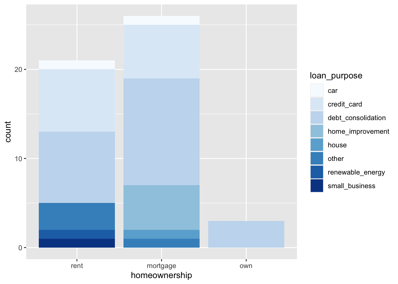
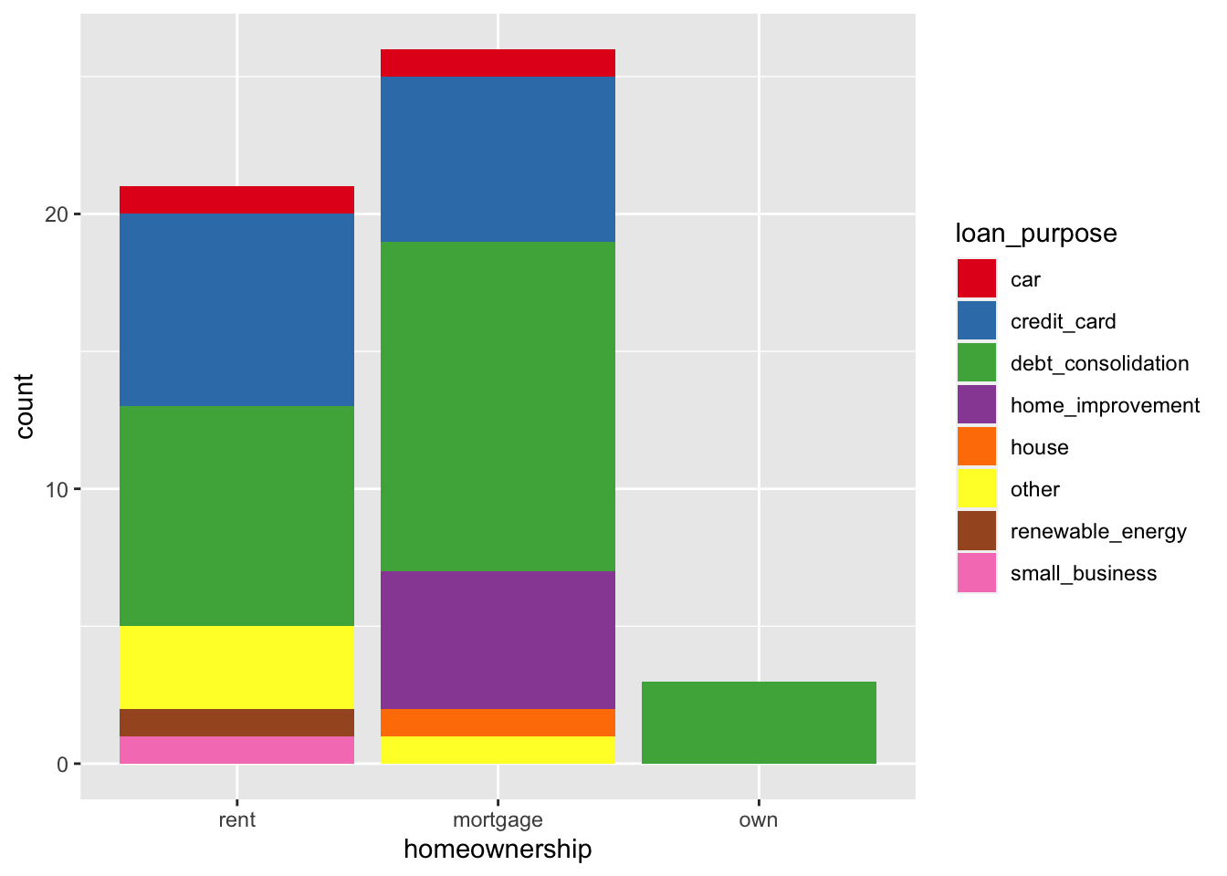
The above looks better but is misleading because it implies an ordinal relationship between the loan purposes and there is no such relationship. We would be better of specifying that the loan_purpose variable is qualitative.
I find the above palette to be ugly but several others are available. Google colorbrewer for more info. By the way, these colors have been extensively psychologically tested to verify that people can easily distinguish between them. I’m uncertain about colorblind people because the most prevalent form of color blindness is red-green.
Now remove the 10th through 85th observations. What is the range, mean, and standard deviation of each predictor in the subset of the data that remains?
Several functions allow you to check up on many columns at once. This is especially helpful in examining dataframes with large numbers of columns, such as amesHousing2011.csv.
$MSSubClass

 020  030  040  045  050  060  070  075  080  085  090  120  150  160  180  190
1078  139    6   18  287  571  128   23  118   48  109  192    1  129   17   61

$MSZoning

A (agr) C (all)      FV I (all)      RH      RL      RM
      2      25     139       2      27    2268     462

$Street

Grvl Pave
  12 2913

$Alley

Grvl Pave
 120   78

$LotShape

 IR1  IR2  IR3  Reg
 975   76   15 1859

$LandContour

 Bnk  HLS  Low  Lvl
 114  120   60 2631

$Utilities

AllPub NoSeWa NoSewr
  2922      1      2

$LotConfig

 Corner CulDSac     FR2     FR3  Inside
    508     180      85      14    2138

$LandSlope

 Gtl  Mod  Sev
2784  125   16

$Neighborhood

Blmngtn Blueste  BrDale BrkSide ClearCr CollgCr Crawfor Edwards Gilbert  Greens
     28      10      30     108      44     267     103     191     165       8
GrnHill  IDOTRR Landmrk MeadowV Mitchel   NAmes NoRidge NPkVill NridgHt  NWAmes
      2      93       1      37     114     443      69      23     166     131
OldTown  Sawyer SawyerW Somerst StoneBr   SWISU  Timber Veenker
    239     151     125     182      51      48      72      24

$Condition1

Artery  Feedr   Norm   PosA   PosN   RRAe   RRAn   RRNe   RRNn
    92    163   2519     20     38     28     50      6      9

$Condition2

Artery  Feedr   Norm   PosA   PosN   RRAe   RRAn   RRNn
     5     13   2896      4      3      1      1      2

$BldgType

  1Fam 2fmCon Duplex  Twnhs TwnhsE
  2420     62    109    101    233

$HouseStyle

1.5Fin 1.5Unf 1Story 2.5Fin 2.5Unf 2Story SFoyer   SLvl
   314     19   1480      8     24    869     83    128

$RoofStyle

   Flat   Gable Gambrel     Hip Mansard    Shed
     20    2320      22     547      11       5

$RoofMatl

CompShg Membran   Metal    Roll Tar&Grv WdShake WdShngl
   2884       1       1       1      23       9       6

$Exterior1st

AsbShng AsphShn BrkComm BrkFace  CBlock CemntBd HdBoard ImStucc MetalSd Plywood
     44       2       6      88       2     124     441       1     450     221
PreCast   Stone  Stucco VinylSd Wd Sdng WdShing
      1       2      42    1026     419      56

$Exterior2nd

AsbShng AsphShn Brk Cmn BrkFace  CBlock CmentBd HdBoard ImStucc MetalSd   Other
     38       4      22      47       3     124     405      14     447       1
Plywood PreCast   Stone  Stucco VinylSd Wd Sdng Wd Shng
    274       1       6      46    1015     397      81

$MasVnrType

 BrkCmn BrkFace  CBlock    None   Stone
     25     879       1    1751     246

$ExterQual

  Ex   Fa   Gd   TA
 103   35  988 1799

$ExterCond

  Ex   Fa   Gd   Po   TA
  12   67  299    3 2544

$Foundation

BrkTil CBlock  PConc   Slab  Stone   Wood
   311   1244   1305     49     11      5

$BsmtQual

  Ex   Fa   Gd   Po   TA
 253   88 1219    2 1283

$BsmtCond

  Ex   Fa   Gd   Po   TA
   3  104  122    5 2611

$BsmtExposure

  Av   Gd   Mn   No
 417  280  239 1906

$BsmtFinType1

ALQ BLQ GLQ LwQ Rec Unf
429 269 854 154 288 851

$BsmtFinType2

 ALQ  BLQ  GLQ  LwQ  Rec  Unf
  53   68   34   89  106 2494

$Heating

Floor  GasA  GasW  Grav  OthW  Wall
    1  2880    27     9     2     6

$HeatingQC

  Ex   Fa   Gd   Po   TA
1490   92  476    3  864

$CentralAir

   N    Y
 196 2729

$Electrical

FuseA FuseF FuseP   Mix SBrkr
  188    50     8     1  2677

$KitchenQual

  Ex   Fa   Gd   Po   TA
 200   70 1160    1 1494

$Functional

Maj1 Maj2 Min1 Min2  Mod  Sal  Sev  Typ
  19    9   65   70   35    2    2 2723

$FireplaceQu

 Ex  Fa  Gd  Po  TA
 42  75 741  46 599

$GarageType

 2Types  Attchd Basment BuiltIn CarPort  Detchd
     23    1727      36     185      15     782

$GarageFinish

 Fin  RFn  Unf
 723  812 1231

$GarageQual

  Ex   Fa   Gd   Po   TA
   3  124   24    5 2610

$GarageCond

  Ex   Fa   Gd   Po   TA
   3   74   15   14 2660

$PavedDrive

   N    P    Y
 216   62 2647

$PoolQC

Ex Fa Gd TA
 3  2  3  3

$Fence

GdPrv  GdWo MnPrv  MnWw
  118   112   329    12

$MiscFeature

Gar2 Othr Shed TenC
   5    4   95    1

$SaleType

  COD   Con ConLD ConLI ConLw   CWD   New   Oth   VWD    WD
   87     5    26     9     8    12   236     7     1  2534

$SaleCondition

Abnorml AdjLand  Alloca  Family  Normal Partial
    189      12      24      46    2412     242
df |>select(where(is.numeric)) |>map ( summary )
$LotFrontage
   Min. 1st Qu.  Median    Mean 3rd Qu.    Max.    NA's
     21      58      68      69      80     313     490

$LotArea
   Min. 1st Qu.  Median    Mean 3rd Qu.    Max.
   1300    7438    9428   10104   11515  215245

$OverallQual
   Min. 1st Qu.  Median    Mean 3rd Qu.    Max.
      1       5       6       6       7      10

$OverallCond
   Min. 1st Qu.  Median    Mean 3rd Qu.    Max.
      1       5       5       6       6       9

$YearBuilt
   Min. 1st Qu.  Median    Mean 3rd Qu.    Max.
   1872    1954    1973    1971    2001    2010

$`YearRemod/Add`
   Min. 1st Qu.  Median    Mean 3rd Qu.    Max.
   1950    1965    1993    1984    2004    2010

$MasVnrArea
   Min. 1st Qu.  Median    Mean 3rd Qu.    Max.    NA's
      0       0       0     101     164    1600      23

$BsmtFinSF1
   Min. 1st Qu.  Median    Mean 3rd Qu.    Max.    NA's
      0       0     370     438     733    2288       1

$BsmtFinSF2
   Min. 1st Qu.  Median    Mean 3rd Qu.    Max.    NA's
      0       0       0      50       0    1526       1

$BsmtUnfSF
   Min. 1st Qu.  Median    Mean 3rd Qu.    Max.    NA's
      0     219     464     559     801    2336       1

$TotalBsmtSF
   Min. 1st Qu.  Median    Mean 3rd Qu.    Max.    NA's
      0     793     990    1047    1299    3206       1

$`1stFlrSF`
   Min. 1st Qu.  Median    Mean 3rd Qu.    Max.
    334     876    1082    1155    1383    3820

$`2ndFlrSF`
   Min. 1st Qu.  Median    Mean 3rd Qu.    Max.
      0       0       0     334     702    1862

$LowQualFinSF
   Min. 1st Qu.  Median    Mean 3rd Qu.    Max.
      0       0       0       5       0    1064

$GrLivArea
   Min. 1st Qu.  Median    Mean 3rd Qu.    Max.
    334    1126    1441    1494    1740    3820

$BsmtFullBath
   Min. 1st Qu.  Median    Mean 3rd Qu.    Max.    NA's
    0.0     0.0     0.0     0.4     1.0     3.0       2

$BsmtHalfBath
   Min. 1st Qu.  Median    Mean 3rd Qu.    Max.    NA's
    0.0     0.0     0.0     0.1     0.0     2.0       2

$FullBath
   Min. 1st Qu.  Median    Mean 3rd Qu.    Max.
      0       1       2       2       2       4

$HalfBath
   Min. 1st Qu.  Median    Mean 3rd Qu.    Max.
    0.0     0.0     0.0     0.4     1.0     2.0

$BedroomAbvGr
   Min. 1st Qu.  Median    Mean 3rd Qu.    Max.
      0       2       3       3       3       8

$KitchenAbvGr
   Min. 1st Qu.  Median    Mean 3rd Qu.    Max.
      0       1       1       1       1       3

$TotRmsAbvGrd
   Min. 1st Qu.  Median    Mean 3rd Qu.    Max.
      2       5       6       6       7      14

$Fireplaces
   Min. 1st Qu.  Median    Mean 3rd Qu.    Max.
      0       0       1       1       1       4

$GarageYrBlt
   Min. 1st Qu.  Median    Mean 3rd Qu.    Max.    NA's
   1895    1960    1979    1978    2002    2207     159

$GarageCars
   Min. 1st Qu.  Median    Mean 3rd Qu.    Max.    NA's
      0       1       2       2       2       5       1

$GarageArea
   Min. 1st Qu.  Median    Mean 3rd Qu.    Max.    NA's
      0     320     480     472     576    1488       1

$WoodDeckSF
   Min. 1st Qu.  Median    Mean 3rd Qu.    Max.
      0       0       0      93     168    1424

$OpenPorchSF
   Min. 1st Qu.  Median    Mean 3rd Qu.    Max.
      0       0      27      47      70     742

$EnclosedPorch
   Min. 1st Qu.  Median    Mean 3rd Qu.    Max.
      0       0       0      23       0    1012

$`3SsnPorch`
   Min. 1st Qu.  Median    Mean 3rd Qu.    Max.
      0       0       0       3       0     508

$ScreenPorch
   Min. 1st Qu.  Median    Mean 3rd Qu.    Max.
      0       0       0      16       0     576

$PoolArea
   Min. 1st Qu.  Median    Mean 3rd Qu.    Max.
      0       0       0       2       0     800

$MiscVal
   Min. 1st Qu.  Median    Mean 3rd Qu.    Max.
      0       0       0      45       0   15500

$MoSold
   Min. 1st Qu.  Median    Mean 3rd Qu.    Max.
      1       4       6       6       8      12

$YrSold
   Min. 1st Qu.  Median    Mean 3rd Qu.    Max.
   2006    2007    2008    2008    2009    2010

$SalePrice
   Min. 1st Qu.  Median    Mean 3rd Qu.    Max.
  12789  129500  160000  180412  213500  625000
Using the above functions would let you quickly and easily to determine that you should delete some columns and convert others to factor or integer. You can delete columns by saying, for instance,
df <- df |>select(-c("Order","PID"))
You may add as many names to the list in the -c() vector as desired.
You may wish to delete columns with a lot of NAs rather than deleting rows with lots of NAs. (Why is this?)
This is easy to discover in the case of numerical columns. For instance, LotFrontage has 490 NAs. You can quickly see that in the output of the above summary. But it doesn’t work for character data. One quick way to see the number of NAs in all columns is to say
Create a Quarto document called week02exercises.qmd. Use your name as the author name and the date as the current date. Make the title within the document “Week 2 Exercises”.
Answer the following questions in the document, using a combination of narration and R chunks.
Use the loan50 data set. Find the mean and median of annual_income using R. Tell why they differ in words.
Use the loan50 data set. Make a contingency table of loan_purpose and grade. Tell the most frequently occurring grade and most frequently occurring loan purpose in words.
Use the loan50 data set. Provide a statistical summary of total_credit_limit.
Use the loan50 data set. Show the column means for all numeric columns.
Use the loan50 data set. Make a contingency table of state and homeownership. Tell which state has the most mortgages in words.
Now render the document and submit both the .qmd file and the .html file to Canvas under “week02exercises”.
2.9.4 Solutions to exercises
Use the loan50 data set. Find the mean and median of annual_income using R. Tell why they differ in words.
They differ because the mean is susceptible to outliers. There are about four outliers in this data set (high annual incomes) and they drag the mean upward but not the median. The median is a more reliable measure of centrality when there are influential outliers.
Use the loan50 data set. Make a contingency table of loan_purpose and grade. Tell the most frequently occurring grade and most frequently occurring loan purpose in words.
#. same info with commas in numbersloan50 |>summarise(Min=comma(min(total_credit_limit)),firstq=comma(quantile(total_credit_limit,0.25)),Median=comma(median(total_credit_limit)),Mean=comma(mean(total_credit_limit)),thirdq=comma(quantile(total_credit_limit,0.75)),Max=comma(max(total_credit_limit)))
     Min firstq  Median    Mean  thirdq     Max
1 15,980 70,526 147,364 208,547 299,766 793,009
Use the loan50 data set. Show the column means for all numeric columns.
Use the loan50 data set. Make a contingency table of state and homeownership. Tell which state has the most mortgages in words.
with(loan50,table(state,homeownership))
     homeownership
state rent mortgage own
         0        0   0
   AK    0        0   0
   AL    0        0   0
   AR    0        0   0
   AZ    0        0   1
   CA    7        2   0
   CO    0        0   0
   CT    1        0   0
   DC    0        0   0
   DE    0        0   0
   FL    1        2   0
   GA    0        0   0
   HI    1        1   0
   ID    0        0   0
   IL    3        0   1
   IN    0        1   1
   KS    0        0   0
   KY    0        0   0
   LA    0        0   0
   MA    1        1   0
   MD    2        1   0
   ME    0        0   0
   MI    0        1   0
   MN    0        1   0
   MO    0        1   0
   MS    0        1   0
   MT    0        0   0
   NC    0        0   0
   ND    0        0   0
   NE    0        1   0
   NH    1        0   0
   NJ    2        1   0
   NM    0        0   0
   NV    0        2   0
   NY    1        0   0
   OH    0        1   0
   OK    0        0   0
   OR    0        0   0
   PA    0        0   0
   RI    0        1   0
   SC    0        1   0
   SD    0        0   0
   TN    0        0   0
   TX    0        5   0
   UT    0        0   0
   VA    1        0   0
   VT    0        0   0
   WA    0        0   0
   WI    0        1   0
   WV    0        1   0
   WY    0        0   0
Texas has five mortgages, more than any other state.
2.9.5 Exercise Notes
Many students did not follow instructions on file naming. I will take off a lot of points if this happens when you turn in a graded assignment. I expect all files to be uniformly named.
Several students left the boilerplate verbiage in their .qmd file. I will take off a lot of points if this happens when you turn in a graded assignment.
One student put their narrative inside the code chunks as R comments. Don’t do this. It undercuts the purpose of mixing narrative and code in a Quarto document.
Some students didn’t try to answer the second part of question 1. One way to understand this is to draw a boxplot of the data, showing that there are four outliers at the top end, dragging the mean upward but leaving the median pretty much alone.
Some students included graphics, which don’t show up in the copy on Canvas. One way to make these graphics show up is to add the following code to the front matter (the front matter is the stuff between two sets of three dashes at the beginning of the file):
format:
  html:
    embed-resources: true
The indentation shown above is essential for it to work.
Some students highlighted relevant rows and columns as shown below. This was a really great addition.
tbl <-with(loan50,table(loan_purpose,grade))tbl <-addmargins(tbl)pacman::p_load(kableExtra)tbl |>kbl() |>kable_classic(full_width=F) |>row_spec(4, color ="white", background ="#AAAAAA") |>column_spec(4, color ="white", background ="#AAAAAA") |>column_spec(1, color ="black", background ="white")
Now you can plug maxrownum and maxcolnum into the formula without having to know which row and column you’re talking about.
tbl |>kbl() |>kable_classic(full_width=F) |>row_spec(maxrownum, color ="white", background ="#AAAAAA") |>column_spec(maxcolnum, color ="white", background ="#AAAAAA") |>column_spec(1, color ="black", background ="white")
A
B
C
D
E
F
G
Sum
0
0
0
0
0
0
0
0
0
car
0
0
1
1
0
0
0
0
2
credit_card
0
6
4
1
1
1
0
0
13
debt_consolidation
0
2
9
4
7
1
0
0
23
home_improvement
0
1
4
0
0
0
0
0
5
house
0
0
1
0
0
0
0
0
1
major_purchase
0
0
0
0
0
0
0
0
0
medical
0
0
0
0
0
0
0
0
0
moving
0
0
0
0
0
0
0
0
0
other
0
4
0
0
0
0
0
0
4
renewable_energy
0
1
0
0
0
0
0
0
1
small_business
0
1
0
0
0
0
0
0
1
vacation
0
0
0
0
0
0
0
0
0
wedding
0
0
0
0
0
0
0
0
0
Sum
0
15
19
6
8
2
0
0
50
And, in the narrative you can say that the maximum frequency of loan_purpose is 23. In the narrative you can alo say that the maximum frequency of grade is 19.
One student stipulated that the mean and median could not ever be the same except in two unusual circumstances. Actually it is quite easy for the mean to equal the mean as you can see from this simple example.