This is a Quarto document. It has three parts: a header, some text written in markdown, and some chunks of R code.
The header of the document contains key-value pairs that are acted upon when the document is rendered to html using the render button. The header is written in a markup language called YAML. YAML cares about indentation, so you need to indent certain items consistently for them to be understood by the renderer.
The main body of the document is text written in Markdown. Markdown was originally written as a kind of shorthand for html so that instead of long html tags, you would use short Markdown tags. For example, this section is called Intro and at the top of it there is a blank line followed by a hashtag followed by the word Intro. You could instead use the html tag <h1>Intro</h1> but it is shorter to write # Intro. For a second level heading you use two hashtags. Keep in mind that you can mix html and Markdown in a Markdown file.
The third part of the document is chunks of R code. These start with a blank line followed by three backticks, followed by the letter r in curly braces. It looks like this:
```{r}1 + 1```
Bear in mind that a backtick is not the same thing as an apostrophe. On your keyboard it is usually on the same key as the tilde.
By default, when you render the document, the code in chunks is executed and the result is displayed in the html version of the document.
1.1 Introducing R and RStudio
First we introduce R and RStudio and, finally, Quarto. First, either use the RStudio server at https://rstudio.ischool.utexas.edu or install R and RStudio, in that order. Some people have trouble installing, especially Windows or Mac. Some Mac users were opening the .dmg file for RStudio as a readonly volume, then open the app on that volume. Instead, you have to drag the RStudio icon to the Applications folder and open it from there. The telltale sign of this problem is that you can’t save any files. Windows users have a different problem. Some Windows users try to install RStudio and R on OneDrive. RStudio won’t run from OneDrive and some Windows users can’t tell the difference between installing on a local hard drive and installing in the cloud on OneDrive.
1.2 Console
The first thing we can try (after installing if you chose to have it on your machine) is to use the console. By default, that is in the lower left of the RStudio window (you can move everything around, though) and it has a command prompt that looks like >. There enter the following function to verify that you can download R packages, which are collections of functions.
install.packages("pacman")
Installing package into '/Users/mcq/Library/R/x86_64/4.3/library'
(as 'lib' is unspecified)
The downloaded binary packages are in
    /var/folders/v2/swcrq0fj2fn4f5lfk896w8g00000gn/T//RtmpZugVo3/downloaded_packages
pacman::p_load(MASS)
If this works, you won’t get any output from the p_load() function but the command prompt will reappear. That function loads the package from the library into our environment so we can use it in the current session. If you screw around with RStudio and particularly if you follow a lot of hints on Stack Overflow, you may end up with several libraries of packages, all out of sync with each other. If you have trouble loading packages from the library, you may want to call the following function to see how many libraries are on your computer and where they are. This function will return the list of library folders on the server if you call it there.
This function returns a list of folders containing libraries, one library per folder. You can then use the terminal or a file explorer outside of R to delete some duplicate packages. You probably have a personal library and a system library at the least.
After loading the relative small package known as MASS, go on to install a package that is actually a large set of packages, collectively known as the Tidyverse. This is a set of packages we will use in our homework.
pacman::p_load(tidyverse)
This takes a while because there are so many packages involved.
1.3 The mtcars data set
There is a lot of data built into R by default. We look at one such data set, called mtcars. Run a function that looks at the first few lines of the data set, head(mtcars), then checked the help screen for the data set, saying help(mtcars), then produce a linear model of the mpg column being predicted by the disp column, saying summary(lm(mpg~disp,data=mtcars)). This linear model is the heart of regression analysis and one of the main things we’ll learn in this course is how to read the summary.
Descriptive statistics deals with numerical analysis of data, such as finding the mean, median etc of values in the dataset. We will find mean, median and mode using the weight column in mtcars with the functions mean() and median(). R doesn’t have a built-in function for mode so we calculate it explicitly.
Histograms show distribution of data. Let’s create a histogram using the data in mtcars. First load the dataset using data(mtcars). Then we use the hist() function in R to create a histogram for the mpg variable.
data(mtcars)hist(mtcars$mpg, main ="Miles per Gallon Distribution", xlab ="Miles per Gallon", ylab ="Frequency")
Then we calculate the range of miles per gallon from the histogram using the range() function.
mpg_range <-range(mtcars$mpg)mpg_range
[1] 10.4 33.9
Now, we will produce a linear model of the mpg column being predicted by the disp column, saying summary(lm(mpg~disp,data=mtcars)). This linear model is the heart of regression analysis and one of the main things we’ll learn in this course is how to read the summary.
summary(lm(mpg~disp,data=mtcars))
Call:
lm(formula = mpg ~ disp, data = mtcars)

Residuals:
    Min      1Q  Median      3Q     Max
-4.8922 -2.2022 -0.9631  1.6272  7.2305

Coefficients:
             Estimate Std. Error t value Pr(>|t|)
(Intercept) 29.599855   1.229720  24.070  < 2e-16 ***
disp        -0.041215   0.004712  -8.747 9.38e-10 ***
---
Signif. codes:  0 '***' 0.001 '**' 0.01 '*' 0.05 '.' 0.1 ' ' 1

Residual standard error: 3.251 on 30 degrees of freedom
Multiple R-squared:  0.7183,    Adjusted R-squared:  0.709
F-statistic: 76.51 on 1 and 30 DF,  p-value: 9.38e-10
1.4 Textbook data sets
Our textbook, Openintro Stats, contains references to a lot of data sets, many of which I’ve downloaded and put into the folder /home/mm223266/data/. You can just use them from this location or go to the URL https://openintro.org/data, but if you can’t remember that, you can just google openintro stats and navigate to the data sets. Look at the metadata for the loan50 data set, which is used in Chapter 1 of the textbook. You can download it in four different formats, the best of which is the .rda file or R Data file. It’s the best because it preserves the data types, in this case dbl, int, and fctr. If we instead import the .csv file, we have to then specify the data types in R, which is an extra step we’d like to avoid when possible.
When we download a file, R doesn’t know where it is automatically. We do one of three things.
Change R to address the folder where we downloaded it
Move it to the folder R is currently addressing
Keep R addressing your homework folder, but reach out for the data sets where I’ve downloaded them (only works if you’re using the RStudio Server).
How you do this depends on the operating system but, in any operating system we use the following three functions.
The first function tells us which folder (or directory if you prefer) R is addressing. The second one changes to the folder / directory we would like to use. (I’ve commented it out for this study guide.) The third one addresses the data where I’ve put it but leaves your working directory where it is. This is very convenient because it means that (1) you don’t have to download data sets, and (2) I don’t have to modify your homework file in order to check it.
My suggestion is that you create a folder for this class and use the third option. You can make your folder your default in RStudio, using Tools > Global Options > General > Default working directory.
Once we load loan50.rda, look at it and try to predict total_credit_limit using annual_income. Keep in mind that, if the file is in the current working directory / folder, R will autocomplete its name when you say lo and then press the tab key (assuming there are no other files starting with the letters lo in the same folder). You just have to enter enough letters to make the name unique before you press the tab key. If nothing happens when you press the tab key, you are either in the wrong folder or you have other files starting with the same letters.
head(loan50)
  state emp_length term homeownership annual_income verified_income
1    NJ          3   60          rent         59000    Not Verified
2    CA         10   36          rent         60000    Not Verified
3    SC         NA   36      mortgage         75000        Verified
4    CA          0   36          rent         75000    Not Verified
5    OH          4   60      mortgage        254000    Not Verified
6    IN          6   36      mortgage         67000 Source Verified
  debt_to_income total_credit_limit total_credit_utilized
1      0.5575254              95131                 32894
2      1.3056833              51929                 78341
3      1.0562800             301373                 79221
4      0.5743467              59890                 43076
5      0.2381496             422619                 60490
6      1.0770448             349825                 72162
  num_cc_carrying_balance       loan_purpose loan_amount grade interest_rate
1                       8 debt_consolidation       22000     B         10.90
2                       2        credit_card        6000     B          9.92
3                      14 debt_consolidation       25000     E         26.30
4                      10        credit_card        6000     B          9.92
5                       2   home_improvement       25000     B          9.43
6                       4   home_improvement        6400     B          9.92
  public_record_bankrupt loan_status has_second_income total_income
1                      0     Current             FALSE        59000
2                      1     Current             FALSE        60000
3                      0     Current             FALSE        75000
4                      0     Current             FALSE        75000
5                      0     Current             FALSE       254000
6                      0     Current             FALSE        67000
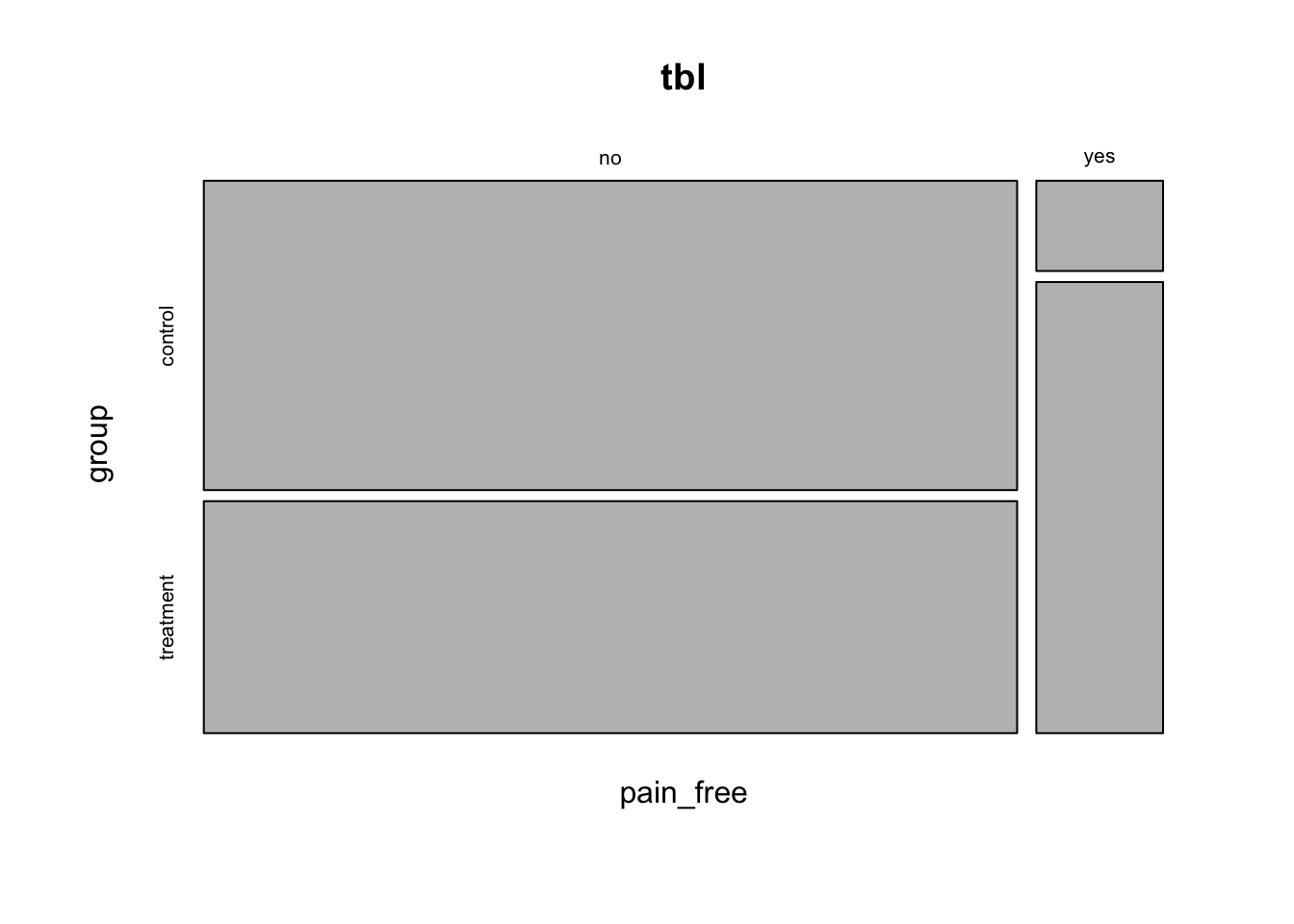
Examine the mosaic plot and the table to see how the sizes of the rectangles compare to the numbers.
We could also more precisely reproduce the figure from the textbook by adding row and column sums.
addmargins(tbl)
         group
pain_free control treatment Sum
      no       44        33  77
      yes       2        10  12
      Sum      46        43  89
We could make it prettier by using the pander package.
pacman::p_load(pander)pander(addmargins(tbl))
control
treatment
Sum
no
44
33
77
yes
2
10
12
Sum
46
43
89
pander has a lot of options we could use to make it even prettier, but we’ll skip that for now. There are also a lot of other packages similar to pander for prettifying R output.
We could display proportions instead of the raw numbers, but it looks ugly, so we’ll then use the options() function to make it look better.
prop.table(tbl)
         group
pain_free    control  treatment
      no  0.49438202 0.37078652
      yes 0.02247191 0.11235955
options(digits=1)prop.table(tbl)
         group
pain_free control treatment
      no     0.49      0.37
      yes    0.02      0.11
Bear in mind that digits=1 is a suggestion to R and that R will determine the exact number of digits on its own, depending on the value of the variables to be displayed.