Stats:
Linear Regression

Mick McQuaid

2024-03-20

Week NINE

Homework

Linear Regression

Finally, the heart of the course

The prediction line on the right is better than that on the left by an amount proportional to the difference between the total length of red lines in the two pictures.

The prediction line is the main component of a linear regression model. Our goal is to do two things: (1) find the best prediction line, and (2) assess it. Bear in mind that the best line may not be very good.

Bear in mind also that we always put the thing we’re trying to predict on the y-axis and the thing we’re using to make the prediction on the x-axis. The x-axis term is typically an input, while the y-axis term is an output.

Basis for the prediction line

\[ y=\beta_0 + \beta_1 x + \epsilon \]

(pronounced y equals beta nought plus beta one x plus epsilon)

This is the idealized regression equation. \(\beta_0\) is the y-intercept of the prediction line and \(\beta_1\) is the slope of the line. \(\epsilon\) is called random error, but that doesn’t mean it’s a mistake. Here the word error simply means a divergence from what the model would otherwise predict. The values of beta are unknown and have to be estimated. The value of epsilon is unknown and we have to make assumptions about it to validate the model.

What we actually see

We see sample data and estimate the preceding equation using data. The estimated regression equation is

\[ \hat{y}=b_0+b_1x \]

Notice that there’s no epsilon. We assume that the mean of the epsilon values is zero. (And we’ll learn how to check that later.)

Names of the variables

\(x\): explanatory variable, predictor, input

\(y\): response, output

Example from textbook: brushtail possums

The textbook gives the regression equation for a model predicting the head length of a brushtail possum given its overall length as follows:

\[ \hat{y}=41+0.59x \]

In other words, the head length is 41mm plus a fraction 0.59 of the total length.

Using R to find the equation

load("possum.rda")
(m <- lm(possum$head_l ~ possum$total_l))

Call:
lm(formula = possum$head_l ~ possum$total_l)

Coefficients:
   (Intercept)  possum$total_l  
       42.7098          0.5729  

For some unknown reason, we would like to estimate the head length of the possums given their total length. The data given on the website differs a little from the data used in the book. The regression equation we give to R separates the output (always comes first) from the input with a tilde or \(\sim\).

Remember epsilon? Now a new term, residual

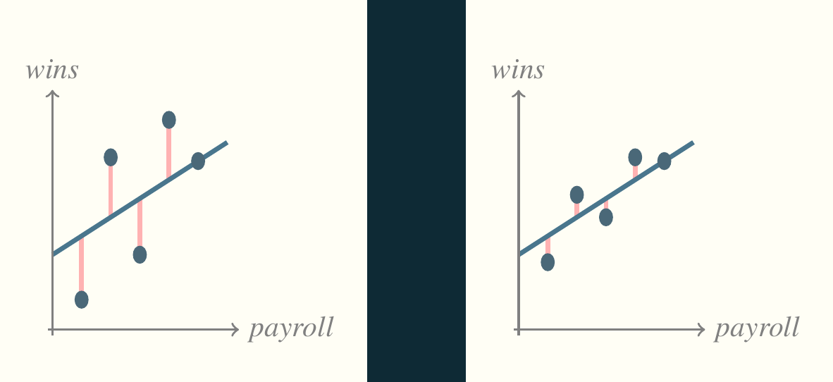
The term epsilon or \(\epsilon\) in the idealized regression equation refers to the divergence of each point from what the model predicts. It’s the pink line in our initial pictures. In the above regression models, each divergence of a single point is called a residual.

Assessing a model with residuals

Think back to the first picture (reproduced below). The residuals are the key to assessing the model.

The total magnitude of the pink lines gives an indication of how good the model is. The model on the left happens to be worse because there’s less of a relationship between wins and payroll than in the model on the right.

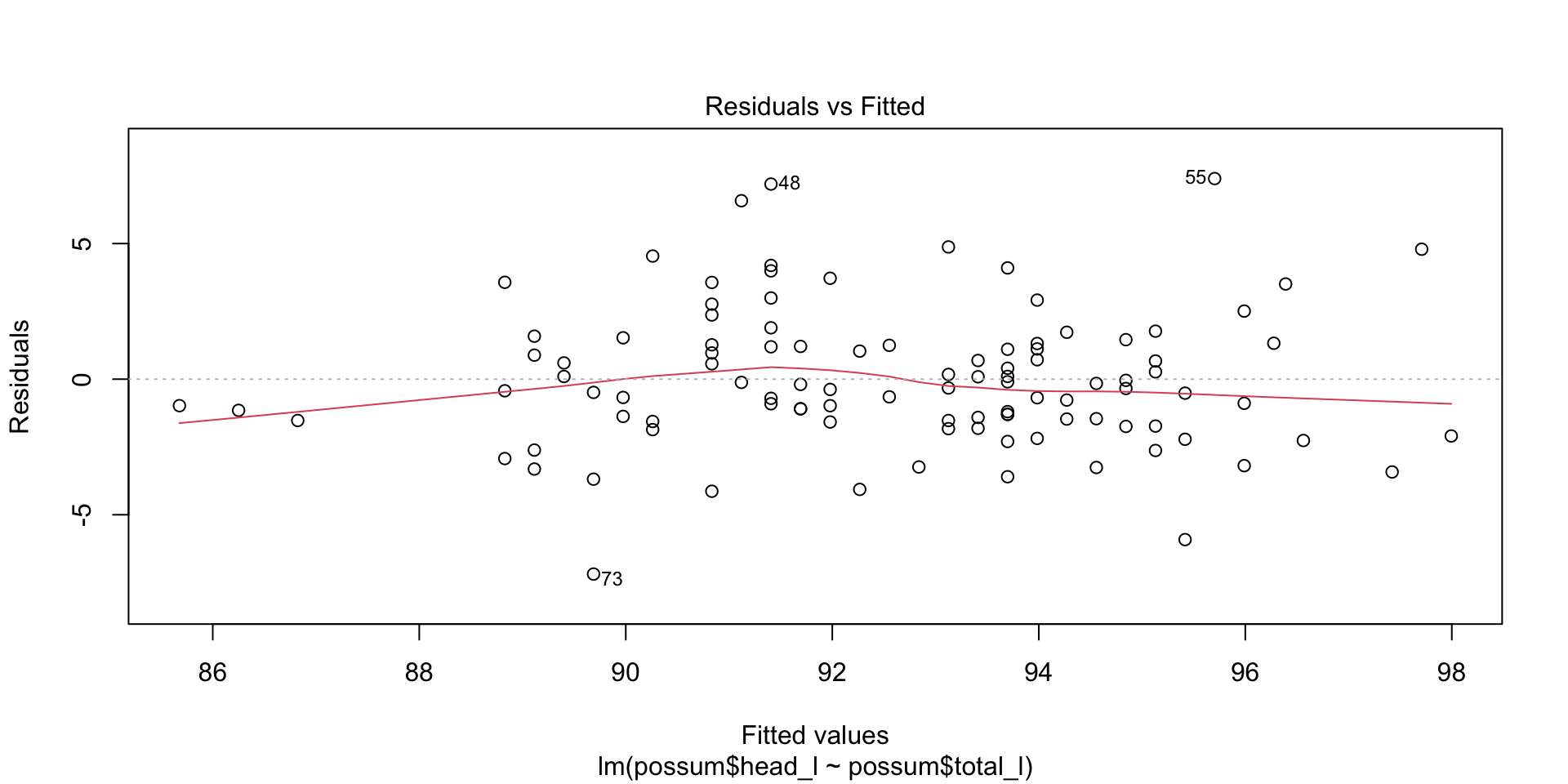
Plotting the residuals

plot(m, which=c(1,1))

This is one of four diagnostic plots that R provides by default when you construct a linear model. What we are looking for in this plot is the absence of a clear pattern. A clear pattern might be a diagonal shift or the cross section of a trumpet.

Correlation

Correlation is a number in the interval \([-1,1]\) describing the strength of the linear association between two variables. The most common measure of correlation (and the only one our textbook bothers to mention) is Pearson’s correlation coefficient, \(r\).

\[r = \frac{1}{n-1}\sum_{i=1}^{n}\frac{x_i-\bar{x}}{s_x}\frac{y_i-\bar{y}}{s_y}\]

Values of \(r\)

\(r=-1\) means that two variables are perfectly negatively correlated.

\(r=0\) means that two variables are completely uncorrelated.

\(r=1\) means that two variables are perfectly positively correlated.

Little r and big R

Every other textbook I’ve ever seen makes a distinction between \(r\), Pearson’s correlation coefficient, and \(R\), the square root of the multiple coefficient of determination. Our textbook, Diez, Çetinkaya-Rundel, and Barr (2019), does not. That’s kind of okay if there is only one predictor, \(x\). It won’t work later when we study multiple regression and assume that more than one input affects the output.

Keep in mind that, in the R language, \(R\) always refers to the square root of the multiple coefficient of determination, which happens to be the same as for \(r\) if there is only one predictor variable.

As an example, I’ve used Mendenhall and Sincich (2012) to learn about regression.

Correlation exercises

Page 314ff of the textbook includes some correlation exercises we can do.

Least squares

How did we arrive at the estimates for slope and intercept? We used a time-honored technique called least squares, which has been around for about two hundred years. It consists of minimizing the sum of squares of the residuals, which are often abbreviated as SSR, SSE, or RSS. To use this technique, we have to make some assumptions and can then use two equations to find the slope and intercept.

Assumptions

• linearity: the data should follow a linear trend—there are advanced regression methods for non-linear relationships
• normality of residuals: The residuals are approximately normally distributed (evaluated with a QQ plot)
• constant variability: The residuals don’t follow a pattern (the most common being a right-facing trumpet)
• independent observations: Usually don’t apply least squares to seasonal data, for example, because its structure can be modeled as a time series

Least squares equations

\[ b_1=\frac{s_y}{s_x}r\]

\[b_0=\bar{y}-b_1\bar{x}\]

Interpreting slope and intercept

Slope: how much \(y\) grows or shrinks for a one-unit increase in \(x\)

Intercept: how large \(y\) would be if \(x\) were 0 (only works if \(x\) can be zero)

If \(b_1\) is positive, \(y\) grows by \(b_1\) if you add one to \(x\). If \(b_1\) is negative, \(y\) shrinks by \(b_1\) if you add one to \(x\). For example, a brushtail possum’s head is 0.59mm longer for every mm the total length increases.

\(b_0\) is the value of \(y\) when \(x=0\). For example, if a brushtail possum’s total length is zero, its head is about 42mm long. This is obviously absurd. You shouldn’t extrapolate outside the bounds of the data you have.

The most common measure of fit

\(r\) is in the interval \([-1,1]\) but \(R^2\) is in the interval \([0,1]\) so \(R^2\) the multiple coefficient of determination represents the proportion of variability in the data that is explained by the model. The adjusted \(R^2\) accounts for a problem with \(R^2\) that we will discuss later. In the case of simple linear regression there is almost no difference.

Example of \(R^2\) for brushtail possum regression

summary(m)

Call:
lm(formula = possum$head_l ~ possum$total_l)

Residuals:
    Min      1Q  Median      3Q     Max 
-7.1877 -1.5340 -0.3345  1.2788  7.3968 

Coefficients:
               Estimate Std. Error t value Pr(>|t|)    
(Intercept)    42.70979    5.17281   8.257 5.66e-13 ***
possum$total_l  0.57290    0.05933   9.657 4.68e-16 ***
---
Signif. codes:  0 '***' 0.001 '**' 0.01 '*' 0.05 '.' 0.1 ' ' 1

Residual standard error: 2.595 on 102 degrees of freedom
Multiple R-squared:  0.4776,    Adjusted R-squared:  0.4725 
F-statistic: 93.26 on 1 and 102 DF,  p-value: 4.681e-16

Categorical variables with two categories

For linear regression, we can NEVER use categorical variables as \(y\), but we often use them as \(x\). The textbook gives an example of sales of Mario Kart game cartridges, where the variable cond takes on the categories new and used. The following frame is a regression of total price (total_pr) on condition (cond).

Categorical variable example

load("mariokart.rda")
(m<-lm(mariokart$total_pr ~ mariokart$cond))

Call:
lm(formula = mariokart$total_pr ~ mariokart$cond)

Coefficients:
       (Intercept)  mariokart$condused  
            53.771              -6.623  

Summary of the preceding model

summary(m)

Call:
lm(formula = mariokart$total_pr ~ mariokart$cond)

Residuals:
    Min      1Q  Median      3Q     Max 
-18.168  -7.771  -3.148   1.857 279.362 

Coefficients:
                   Estimate Std. Error t value Pr(>|t|)    
(Intercept)          53.771      3.329  16.153   <2e-16 ***
mariokart$condused   -6.623      4.343  -1.525     0.13    
---
Signif. codes:  0 '***' 0.001 '**' 0.01 '*' 0.05 '.' 0.1 ' ' 1

Residual standard error: 25.57 on 141 degrees of freedom
Multiple R-squared:  0.01622,   Adjusted R-squared:  0.009244 
F-statistic: 2.325 on 1 and 141 DF,  p-value: 0.1296

The summary tells us a few things. This is a case where \(x=0\) is valid because it means that the game is new. So a new game is worth 53.77 USD, while being used subtracts 6.62 USD from its value. On the other hand, it is a terrible model based on the small \(R^2\), the small F-statistic (more on that later), and the F-statistic’s large p-value.

Least squares exercises

Page 325 has some exercises we can try.

Outliers

Page 329 shows six different kinds of outliers, while page 328 has a description of them. Do you agree with the textbook assessment?

Leverage

Points far from the horizontal center have high leverage, in the sense that they can pull the regression line up or down more forcefully than can outliers near the horizontal center.

Influential points

A subset of high leverage points are those that actually exercise this high leverage and do pull the regression line out of position.

It can be dangerous to remove these points from analysis for reasons explored in a book called The Black Swan.

Software

Let’s examine the models we generated previously.

summary(m)

Call:
lm(formula = mariokart$total_pr ~ mariokart$cond)

Residuals:
    Min      1Q  Median      3Q     Max 
-18.168  -7.771  -3.148   1.857 279.362 

Coefficients:
                   Estimate Std. Error t value Pr(>|t|)    
(Intercept)          53.771      3.329  16.153   <2e-16 ***
mariokart$condused   -6.623      4.343  -1.525     0.13    
---
Signif. codes:  0 '***' 0.001 '**' 0.01 '*' 0.05 '.' 0.1 ' ' 1

Residual standard error: 25.57 on 141 degrees of freedom
Multiple R-squared:  0.01622,   Adjusted R-squared:  0.009244 
F-statistic: 2.325 on 1 and 141 DF,  p-value: 0.1296

The coefficents table

There are five columns in the coefficients table

• Estimate: the coefficient estimate (\(b_0, b_1\)) of the parameter (\(\beta_0,\beta_1\))
• Std Error: the standard error of the coeffient (stdev scaled by sample size)
• t value: the ratio of the estimate to its standard error
• Pr(>|t|): the p-value of the t-statistic
• Significance codes (unlabeled): category the p-value falls into

Hypothesis tests

The coefficients table tells us all we need to know to conduct a hypothesis test concerning an estimate, where the hypothesis is typically whether the true value of the coefficient is zero. If it is zero, the input variable associated with the coefficient is not linearly related to the output or response variable.

Confidence intervals

By default, R gives a ninety-five percent confidence interval for all coefficients. Notice that condition: used includes zero, highlighting the unreliability of the estimate.

confint(m)

                       2.5 %    97.5 %
(Intercept)         47.18973 60.351630
mariokart$condused -15.20910  1.963936

Computing confidence intervals by hand

\[b_i \pm t^*_{df} \times SE_{b_i}\]

For the mariokart model, \(t^*_{df}\) can be found for the ninety-five percent confidence interval by

qt(0.975,141)

[1] 1.976931

and \(b_i\) and \(SE_{b_i}\) are given in the coefficients table.

Inference for linear regression exercises

Page 335 of the textbook has exercises in inference we can try.

END

References

Diez, David, Mine Çetinkaya-Rundel, and Cristopher D Barr. 2019. OpenIntro Statistics, Fourth Edition. self-published. https://openintro.org/os.

Mendenhall, William, and Terry Sincich. 2012. A Second Course in Statistics, Regression Analysis, Seventh Edition. Boston, MA, USA: Prentice Hall.

Colophon

This slideshow was produced using quarto

Fonts are Roboto Condensed Bold, JetBrains Mono Nerd Font, and STIX2