Statistics: Intro

Mick McQuaid

2024-01-11

Week ONE

uncertainty

Uncertainty is our enemy. Our goal is to reduce uncertainty. An important source of uncertainty is variability in data.

Variability in data

• Your GPA fluctuates
• Your gas mileage fluctuates
• The cost of basic necessities fluctuates

Summarizing data, 1 of 2

We use the mean and standard deviation to summarize many data items

u <- c(1,2,3,4,5)
mean(u)

[1] 3

sd(u)

[1] 1.581139

Summarizing data, 2 of 2

v <- c(2,3,3,3,4)
mean(v)

[1] 3

sd(v)

[1] 0.7071068

\(v\) is less variable than \(u\), even though they are the same on average. We need the standard deviation to know that, although we will later learn some pictures we can draw to illustrate it.

Let’s do some examples on the computer

• Install R (just google the letter R)
• Install R Studio (after installing R)
• Be sure you install these on your local disk, not in the cloud

Now, recreate the above examples

• \(u\) and \(v\) are vectors and can be any size you like
• try using different numbers
• try using prices at different vendors for something you might want to buy or sell
• c() is a function that combines numbers or words into vectors
• The symbol <- can be read as the word gets, as in “\(u\) gets the vector of numbers 1 through 5”

Bundles of vectors called dataframes

• R has built-in dataframes
• One is called mtcars
• Type the word mtcars into the R console and press Enter to see it
• You can find the mean and standard deviation of any given column by saying, e.g., mean(mtcars$mpg)
• The part that says mtcars$ tells R what dataframe to use to find mpg
• Each column of mtcars is a vector

The mtcars dataframe

• The name of each vector is an abbreviation at the top
• The full names can be found by saying ?mtcars which also gives other information about the dataframe
• You can find all the column means by saying colMeans(mtcars)
• You can find all the standard deviations by saying sapply(mtcars,sd)
• The call colMeans(mtcars) is a faster version of sapply(mtcars,mean)

Packages

• Most of the functionality in R is in packages
• You install packages into the library and retrieve them from there
• Some packages are actually collections of packages
• We’ll use a collection called the tidyverse
• So say install.packages("tidyverse") now
• Also say install.packages("pacman") because it simplifies installation and loading

A picture of mtcars

#. install.packages("pacman")
pacman::p_load(tidyverse)
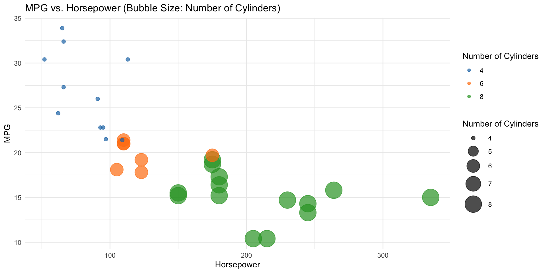
ggplot(mtcars, aes(x = hp, y = mpg, size = cyl, color = factor(cyl))) +
  geom_point(alpha = 0.7) +
  scale_size_continuous(range = c(2, 10)) +
  scale_color_manual(values = c("#1f77b4", "#ff7f0e", "#2ca02c", "#d62728", "#9467bd", "#8c564b", "#e377c2", "#7f7f7f", "#bcbd22", "#17becf")) +
  labs(x = "Horsepower", y = "MPG", size = "Number of Cylinders", color = "Number of Cylinders", title = "MPG vs. Horsepower (Bubble Size: Number of Cylinders)") +
  theme_minimal()

This and several other pictures of the mtcars dataframe can be found at https://rpubs.com/Smruti/1061420

Goal

• Interpret the variability in data
• Describe unwieldly data
• Estimate unknown quantities
• Predict the future
• Understand the mechanisms affecting stochastic processes

This course helps you to interpret the variability in data. The goal is to help you estimate and predict unknown quantities, a common task in business as elsewhere in life. For example, you might try to estimate future sales by taking an average of past sales. You might already have learned how to do that. In this course, you will learn a method that may yield better results. Suppose you know that there is a relationship between advertising and sales. You may be able to form a better estimate of future sales by taking what you know about that relationship into account. The technique you’ll learn here for predicting or estimating a quantity like sales, taking into account what you know about its relationship to another quantity, like advertising, is called regression.

Difference between prediction lines

The prediction line on the right is better than that on the left by an amount proportional to the difference between the total length of red lines in the two pictures.

This course is about finding and assessing the best line

• Consider a desired outcome (e.g., wins)
• Identify one or more factors contributing (e.g., payroll dollars)
• Find the slope and intercept to predict how much of the factor leads to how much of the outcome
• Figure out how good or bad the prediction is

\(\ldots{}\) and there you have a simplified view of regression, the heart of this course.

Think about the prediction lines as models of reality

• reduces reality to a manageable fiction
• requires deep knowledge of the subject you model
• easy to do badly
• hard to figure out what aspects of reality to leave in and what to take out

Modeling

• That’s the process I’ve just described
• Mainly equations of lines in this class
• Parsimonious description of some aspect of reality

The process I’ve just described is a process called modeling. Some people call the equations of lines models. It is more correct though to say that the model includes both the equations and a set of statements related to the equations. When we work with models we need to pause and think about what models are and why we make them.

A model is a parsimonious description of some aspect of reality. The word parsimonious literally means frugal or stingy. In science it means we leave out the aspects of reality that are not absolutely necessary. Opinions differ about what is absolutely necessary.

Expense of modeling

• More realistic \(\Rightarrow\) more expensive
• Example: fishing

The more realistic model is the more expensive it becomes to construct: In business we want to find the minimum amount of stuff we have to keep track of in order to construct a model that useful enough to manage.

People need to make choices and assess how good their choices were. We need models that are good enough to make choices and good enough to help us monitor how our execution of choices is going. Consider a simple example of fishing. When I arrived in a West Coast town, a man told me that within a 50 mile radius there are 300 miles of fishing coastline. He claimed that most people here fish. Do you? Suppose two fishermen each tell you their favorite spot is the best for catching big walleye. It might be impolite to ask them to prove it. One weekend you accompany fisherman Q to his favorite spot and catch some walleye. The polite thing to say is that these are the finest and biggest walleye you have ever seen. When you get home and fisherman Q is not around you weigh the walleye. The next weekend you do the same with fisherman R. The next weekend both fishermen want you to go to their spot at the same time. Both fishermen are equally fun to be around. Both bring the finest cold beer with them. The only difference you can think of is that perhaps one stream has bigger walleye and thus better helps you to feed your family. Which do you choose?

Notice the ways in which this model is not realistic. All this model includes is our location and weight and nothing else. Is that a good description of reality? No two people are equally fun. No two beers are equally cold. No two spots next to streams are equally comfortable. Can you think of more variables we just left out? You should be able to. Much of the art of management is figuring out which variables are important. Some of the art of management is being able to reframe the problem. For example you could perhaps convince both of the fishermen to try a new third spot, even if it is just to prove their spots are better.

Death penalty in Florida example

• Analysts tried to find racism in the death penalty in Florida
• Most failed
• How could they go wrong?
• Finally, one analyst figured it out. How?

Many analysts tried to determine whether the death penalty in Florida was being applied in a racist manner. Many failed to do so. Most tried to predict the likelihood that a murderer would receive the death penalty (\(y\)) as a function of the race of the murderer (\(x\)). Various analysts tried to control for different factors, such as the relative populations of each race from which murderers are convicted. Finally, one analyst considered a different model: predicting the likelihood that a convicted murderer would receive the death penalty (\(y\)) as a function of the race of the victim of the murder (\(x\)). Using this model, the analyst showed that a murderer is overwhelmingly more likely to receive the death penalty for murdering a white victim than for a murdering a victim of color. Why had this seemingly simple model eluded analysts for so many years? The answer, in part, is that modeling is very hard. Choosing the right variables is very hard.

Technicality of this course

• You will learn the mechanics
• You will learn how to build models
• You have to supply the intuition and insight
• No one can teach you to think of the best model

This is a technical course in which you will work with the mechanics of models. Many of the most important issues in modeling are outside the scope of this course. We believe it will take you 14 weeks to figure out the mechanics of building and analyzing regression models. The task of figuring out which models are worthwhile to build and analyze for decision-making purposes may take your whole career.

Summary statistics

Goals for this section

• Distinguish between samples and populations.
• Know how to calculate the arithmetic mean.
• Know how to calculate standard deviation.
• Know the definition of median.
• Review other summary statistics.

This section introduces the mean, the distinction between sample mean and population mean, the range, the sample and population variance, and the sample and population standard deviation. We will also examine the simplest visualization: a stem-and-leaf plot and a set of descriptive statistics, including \(N\), mean, median, Trimmed mean, standard deviation, Standard Error, minimum, maximum, first quartile, and third quartile.

Guidelines for interpreting standard deviation are (a) for any data set, at least three-fourths of the measurements will lie within two standard deviations of the mean, and (b) for most data sets with enough measurements (25 or more) and a mound-shaped distribution, about 95 percent of the measurements will lie within two standard deviations of the mean.

We use samples to make inferences about populations

What you see here are pictures of certificates of testing on shipping boxes. These certificates attest that the boxes are strong. They are legally mandated.

Shipping boxes bear certificates of testing as a benefit of the Uniform Commercial Code, which allows businesses in each of the fifty United States to make legally-binding assumptions about the businesses they work with in other states. If someone ships something to you, you can mandate that it is in a box that has met Uniform Commercial Code requirements, including the fact that it is hard to crush the box. Unfortunately, you have to destroy the box to conduct the crush test.

Therefore a sample of boxes are tested to estimate the parameters of the population of boxes and we need terminology to talk about both sample and population. The next thing we will talk about is that terminology.

finding a sum is denoted like this

The Greek letter Sigma, \(\Sigma\), usually means to sum the values represented by the expression that follows:

\[\sum_{i=1}^n y_i\]

which is the same as

\[y_1 + y_2 + \cdots + y_n\]

The first terminology we’ll see is the Greek letter Sigma, used to denote sums.

Sigma notation may be inconsistent

You may see \(\Sigma\) used in an inconsistent way in math and stats:

\[\sum_{i=1}^n y_i\]

may be replaced by a synonymous shortcut like

\[\sum_{i} y_i \quad \text{or} \quad \sum y\]

Means

The arithmetic mean is the average of a set of values.

Usually when we use the word mean, we refer to

\[ \overline{y} = \frac{\sum_{i=1}^n y_i}{n}\]

which is the same as

\[ \overline{y} = \frac{y_1 + y_2 + \cdots + y_n}{n}\]

Sample mean and population mean

We use the sample mean to estimate the population mean.

The sample mean is often denoted as \(\overline{y}\).

The population mean is called the expected value of \(y\) and is often denoted as

\[E(y)=\mu\]

and in the case of the boxes, we would have to destroy all of them to be sure of its value, so we destroy a sample to estimate \(\mu\).

Range

A sample’s range is the difference between its max and min.

If the grades of a sample of six students are

\[(2, 2, 3, 3, 4, 4)\]

then the range is

\[4-2=2\]

The mean of the sample is \[\overline{y}=(2+2+3+3+4+4)/6=3\]

Standard deviation

Standard deviation is used to describe data variation.

The standard deviation of a population is \(\sigma\) and of a sample is \(s\). It’s painfully easy to confuse the spreadsheet functions for \(\sigma\) and \(s\), usually stdev and sstdev.

\[\sigma=\sqrt{\frac{\sum_{i=1}^n (y_i-\mu)^2}{n}}\]

\[s=\sqrt{\frac{\sum_{i=1}^n (y_i-\overline{y})^2}{n-1}}\]

Standard deviation example

Find the standard deviation of the grade sample.

• sum: \(2+2+3+3+4+4=18\)
• mean: \(18/6=3\)
• deviations: \((2-3)^2+(2-3)^2+(3-3)^2+(3-3)^2+(4-3)^2+(4-3)^2\)
• deviations part two: \(1+1+0+0+1+1\)
• divide: \(4/(6-1)=4/5=0.8\)
• square root: just write \(\sqrt{0.8}\) unless you’re allowed a calculator / computer

Deviations

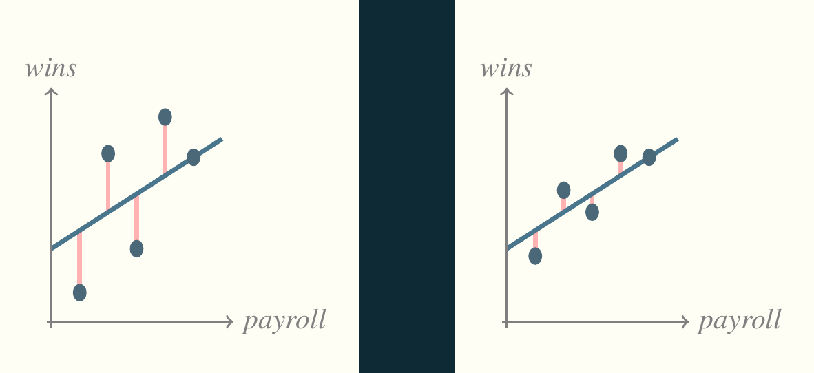
The deviations part two step shown previously is the numerical version of what I previously showed in the graph with pink lines between data and some imaginary prediction line. In this case, the imaginary line is \(\overline{y}\). (In the previous case, it was the least squares line, which we’ll learn about later.)

Standard deviation calculation

Calculating \(s\) emphasizes its interpretation

Here’s a shortcut equivalent to the previous formula for \(s\).

\[s=\sqrt{\frac{\sum_{i=1}^n y_i^2 - n(\overline{y})^2}{n-1}}\]

Previously I asked you to add up the deviations, even though there is a math shortcut that prevents you from having to do so. I asked you to do it this way because the shortcut does not make an obvious connection between the pink lines in the graph at the beginning of the introduction and the result of the equation.

Keep in mind that they give equivalent results. The \(s\) in this equation is the same \(s\) as above.

Two rough guidelines to interpret \(s\)

1. For any data set, at least three-fourths of the measurements will lie within two standard deviations of the mean.
2. For most data sets with enough measurements (25 or more) and a mound-shaped distribution, about 95 percent of the measurements will lie within two standard deviations of the mean. (We’ll study mound-shaped distributions later.)

These are rough guidelines. Confidence intervals and prediction intervals offer much more precise guidelines we’ll learn later but will require that certain assumptions are met. We’ll always use confidence intervals or prediction intervals in preference to these rough guidelines if we can meet these assumptions.

Standard deviation and mean work as a pair.

When you want to describe a set of data, the two most frequently used numbers, used as a pair, are mean and standard deviation. Suppose two websites, tra.com and la.com, both sell used phones. The last five sales of the ZZ11 on tra.com, in chronological order, were $36, $29, $59, $18, $23, $35, $25, $63, $69, and $43.

The last fives sales of the ZZ11 on la.com, in chronological order, were $44, $36, $47, $38, $35, $36, $37, $38, $50, and $39. Using only this info, what is the expected value of the next sale in each market? How is it spread out in each market?

Our best estimate of the expected value is the sample mean, which is $40 in both cases. What about the standard deviation? Calculating the standard deviation will give you about $17.95 for tra.com and $5.16 for la.com. So the most likely value in each market is $40 but we have a lot more confidence in that estimate for la.com. It’s not that we expect a different value. It’s that the values are more widely dispersed in the first case than in the second case. It’s more likely that we’ll get $40 for our used phone if the sale prices are all near $40. If half the sales in bla.com were for $5 and half were for $75, the expected value would still be $40, even though the comparison of the bla.com market to the other two markets provides a striking difference in risk. Which market would you prefer? Surely it would depend in part on how much risk you were willing to absorb. The safe bet would be on the market with a standard deviation of $5.16 and the riskiest would be the bla.com market with a standard deviation of $36.89.

Do it in R

tra <- c(36,29,59,18,23,35,25,63,69,43)
mean(tra)

[1] 40

sd(tra)

[1] 17.95055

la <- c(44,36,47,38,35,36,37,38,50,39)
mean(la)

[1] 40

sd(la)

[1] 5.163978

Further, suppose bla.com has mean 40 and sd 36.89. Where would you sell?

So we conclude this section by saying that the standard deviation really enriches our description of a data set beyond the description given by the mean.

Summary statistics in R

#. help(mtcars)
#. ?mtcars
df <- mtcars
summary(df$mpg)

   Min. 1st Qu.  Median    Mean 3rd Qu.    Max. 
  10.40   15.43   19.20   20.09   22.80   33.90 

(s <- sd(df$mpg))

[1] 6.026948

(m <- mean(df$mpg))

[1] 20.09062

(lower <- m-(2*s))

[1] 8.036729

(upper <- m+(2*s))

[1] 32.14452

Summarize the entire dataframe

str(df)

'data.frame':   32 obs. of  11 variables:
 $ mpg : num  21 21 22.8 21.4 18.7 18.1 14.3 24.4 22.8 19.2 ...
 $ cyl : num  6 6 4 6 8 6 8 4 4 6 ...
 $ disp: num  160 160 108 258 360 ...
 $ hp  : num  110 110 93 110 175 105 245 62 95 123 ...
 $ drat: num  3.9 3.9 3.85 3.08 3.15 2.76 3.21 3.69 3.92 3.92 ...
 $ wt  : num  2.62 2.88 2.32 3.21 3.44 ...
 $ qsec: num  16.5 17 18.6 19.4 17 ...
 $ vs  : num  0 0 1 1 0 1 0 1 1 1 ...
 $ am  : num  1 1 1 0 0 0 0 0 0 0 ...
 $ gear: num  4 4 4 3 3 3 3 4 4 4 ...
 $ carb: num  4 4 1 1 2 1 4 2 2 4 ...

summary(df)

      mpg             cyl             disp             hp       
 Min.   :10.40   Min.   :4.000   Min.   : 71.1   Min.   : 52.0  
 1st Qu.:15.43   1st Qu.:4.000   1st Qu.:120.8   1st Qu.: 96.5  
 Median :19.20   Median :6.000   Median :196.3   Median :123.0  
 Mean   :20.09   Mean   :6.188   Mean   :230.7   Mean   :146.7  
 3rd Qu.:22.80   3rd Qu.:8.000   3rd Qu.:326.0   3rd Qu.:180.0  
 Max.   :33.90   Max.   :8.000   Max.   :472.0   Max.   :335.0  
      drat             wt             qsec             vs        
 Min.   :2.760   Min.   :1.513   Min.   :14.50   Min.   :0.0000  
 1st Qu.:3.080   1st Qu.:2.581   1st Qu.:16.89   1st Qu.:0.0000  
 Median :3.695   Median :3.325   Median :17.71   Median :0.0000  
 Mean   :3.597   Mean   :3.217   Mean   :17.85   Mean   :0.4375  
 3rd Qu.:3.920   3rd Qu.:3.610   3rd Qu.:18.90   3rd Qu.:1.0000  
 Max.   :4.930   Max.   :5.424   Max.   :22.90   Max.   :1.0000  
       am              gear            carb      
 Min.   :0.0000   Min.   :3.000   Min.   :1.000  
 1st Qu.:0.0000   1st Qu.:3.000   1st Qu.:2.000  
 Median :0.0000   Median :4.000   Median :2.000  
 Mean   :0.4062   Mean   :3.688   Mean   :2.812  
 3rd Qu.:1.0000   3rd Qu.:4.000   3rd Qu.:4.000  
 Max.   :1.0000   Max.   :5.000   Max.   :8.000  

Less ugly summaries

pacman::p_load(vtable)
df <- mtcars
df |> sumtable(summ=c('mean(x)','median(x)'),out='return')

   Variable Mean Median
1       mpg   20     19
2       cyl  6.2      6
3      disp  231    196
4        hp  147    123
5      drat  3.6    3.7
6        wt  3.2    3.3
7      qsec   18     18
8        vs 0.44      0
9        am 0.41      0
10     gear  3.7      4
11     carb  2.8      2

There’s just one problem

• Not all of the columns should be numeric
• Discover this by saying ?mtcars in the R console
• You may also say str(mtcars) to discover that all of the columns are currently numeric
• You have to manually change each of columns 2 and 8 through 11 to factors (see next slide)

Changing columns to factors, first way

df[,2] <- as.factor(df[,2])
df[,8] <- as.factor(df[,8])
df[,9] <- as.factor(df[,9])
df[,10] <- as.factor(df[,10])
df[,11] <- as.factor(df[,11])

Changing columns to factors, second way

df |> mutate(across(c(2,8:11),as.factor))

                     mpg cyl  disp  hp drat    wt  qsec vs am gear carb
Mazda RX4           21.0   6 160.0 110 3.90 2.620 16.46  0  1    4    4
Mazda RX4 Wag       21.0   6 160.0 110 3.90 2.875 17.02  0  1    4    4
Datsun 710          22.8   4 108.0  93 3.85 2.320 18.61  1  1    4    1
Hornet 4 Drive      21.4   6 258.0 110 3.08 3.215 19.44  1  0    3    1
Hornet Sportabout   18.7   8 360.0 175 3.15 3.440 17.02  0  0    3    2
Valiant             18.1   6 225.0 105 2.76 3.460 20.22  1  0    3    1
Duster 360          14.3   8 360.0 245 3.21 3.570 15.84  0  0    3    4
Merc 240D           24.4   4 146.7  62 3.69 3.190 20.00  1  0    4    2
Merc 230            22.8   4 140.8  95 3.92 3.150 22.90  1  0    4    2
Merc 280            19.2   6 167.6 123 3.92 3.440 18.30  1  0    4    4
Merc 280C           17.8   6 167.6 123 3.92 3.440 18.90  1  0    4    4
Merc 450SE          16.4   8 275.8 180 3.07 4.070 17.40  0  0    3    3
Merc 450SL          17.3   8 275.8 180 3.07 3.730 17.60  0  0    3    3
Merc 450SLC         15.2   8 275.8 180 3.07 3.780 18.00  0  0    3    3
Cadillac Fleetwood  10.4   8 472.0 205 2.93 5.250 17.98  0  0    3    4
Lincoln Continental 10.4   8 460.0 215 3.00 5.424 17.82  0  0    3    4
Chrysler Imperial   14.7   8 440.0 230 3.23 5.345 17.42  0  0    3    4
Fiat 128            32.4   4  78.7  66 4.08 2.200 19.47  1  1    4    1
Honda Civic         30.4   4  75.7  52 4.93 1.615 18.52  1  1    4    2
Toyota Corolla      33.9   4  71.1  65 4.22 1.835 19.90  1  1    4    1
Toyota Corona       21.5   4 120.1  97 3.70 2.465 20.01  1  0    3    1
Dodge Challenger    15.5   8 318.0 150 2.76 3.520 16.87  0  0    3    2
AMC Javelin         15.2   8 304.0 150 3.15 3.435 17.30  0  0    3    2
Camaro Z28          13.3   8 350.0 245 3.73 3.840 15.41  0  0    3    4
Pontiac Firebird    19.2   8 400.0 175 3.08 3.845 17.05  0  0    3    2
Fiat X1-9           27.3   4  79.0  66 4.08 1.935 18.90  1  1    4    1
Porsche 914-2       26.0   4 120.3  91 4.43 2.140 16.70  0  1    5    2
Lotus Europa        30.4   4  95.1 113 3.77 1.513 16.90  1  1    5    2
Ford Pantera L      15.8   8 351.0 264 4.22 3.170 14.50  0  1    5    4
Ferrari Dino        19.7   6 145.0 175 3.62 2.770 15.50  0  1    5    6
Maserati Bora       15.0   8 301.0 335 3.54 3.570 14.60  0  1    5    8
Volvo 142E          21.4   4 121.0 109 4.11 2.780 18.60  1  1    4    2

Changing columns to factors, third way

df$vs <- factor(df$vs,labels=c("V","S"))
df$am <- factor(df$am,labels=c("automatic","manual"))
df$cyl <- ordered(df$cyl)
df$gear <- ordered(df$gear)
df$carb <- ordered(df$carb)

Structure after repair

str(df)

'data.frame':   32 obs. of  11 variables:
 $ mpg : num  21 21 22.8 21.4 18.7 18.1 14.3 24.4 22.8 19.2 ...
 $ cyl : Ord.factor w/ 3 levels "4"<"6"<"8": 2 2 1 2 3 2 3 1 1 2 ...
 $ disp: num  160 160 108 258 360 ...
 $ hp  : num  110 110 93 110 175 105 245 62 95 123 ...
 $ drat: num  3.9 3.9 3.85 3.08 3.15 2.76 3.21 3.69 3.92 3.92 ...
 $ wt  : num  2.62 2.88 2.32 3.21 3.44 ...
 $ qsec: num  16.5 17 18.6 19.4 17 ...
 $ vs  : Factor w/ 2 levels "V","S": 1 1 2 2 1 2 1 2 2 2 ...
 $ am  : Factor w/ 2 levels "automatic","manual": 2 2 2 1 1 1 1 1 1 1 ...
 $ gear: Ord.factor w/ 3 levels "3"<"4"<"5": 2 2 2 1 1 1 1 2 2 2 ...
 $ carb: Ord.factor w/ 6 levels "1"<"2"<"3"<"4"<..: 4 4 1 1 2 1 4 2 2 4 ...

Less ugly summaries, just the numeric columns

df[,c(1,3:7)] |> sumtable(summ=c('min(x)','median(x)','mean(x)','max(x)'),out='return')

  Variable Min Median Mean Max
1      mpg  10     19   20  34
2     disp  71    196  231 472
3       hp  52    123  147 335
4     drat 2.8    3.7  3.6 4.9
5       wt 1.5    3.3  3.2 5.4
6     qsec  14     18   18  23

It’s tough to make predictions, especially about the future.

— Yogi Berra

As this intro continues, bear in mind that, overall, our goal is to make inferences from data, not an easy task.

END

Colophon

This slideshow was produced using quarto

Fonts are Roboto Condensed Bold, JetBrains Mono Nerd Font, and STIX